Processing Steps
This section describes how to run the key processing steps and what each step does. The previous section describes which of these steps you should run, and in which order, depending on the desired goals. However, processing step are generally run in the order listed below, with some steps only needed for one workflow or another.
Create a New Project
The TeleSculptor application requires a working directory, also called the project folder, in which to save settings and algorithm results when processing a video. To create a new project use the File → New Project menu item or keyboard shortcut Ctrl+N. Create a new empty folder at the desired location and press the “Select Folder” button with that new folder highlighted.
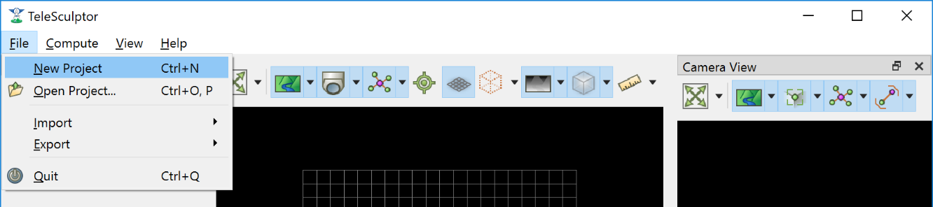
Create a new project from the File->New Project menu item.
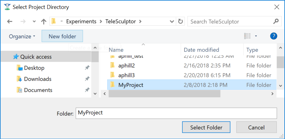
Create a new project folder to store the results of processing.
After creating the new project, the application will create a project file in the project directory with the same name and a “.conf” file extension. In the example shown in the figure above it will create MyProject/MyProject.conf. This conf file is known as the project file or the project configuration file. It contains the configuration settings for the project. To reload an existing project after closing the application, use File->Open and select this project configuration file.
The user must create or open a project before running any of the tools in the Compute menu. The application can open videos and other files for inspection without a project but cannot process the data without a project. The recommended workflow is to create a project first and then open a video, however, if the project is created after opening a video the open video will be added to the new project.
Projects can have any name and refer to a video file at any location on the computer. That said, for better organization we recommend giving the project folder the same name video clip that will be processed. If it is possible to move the video clip into the new project folder before opening the video the project will be relocatable. That is, if the source video is in the project folder you can move the project folder to another location or another computer and it will still load. If the video is outside the project folder the absolute path will be recorded, but this link could become broken if the video or project is moved later.
Import a Video
To import a video clip, use the File->Import->Imagery menu item. In the Open File dialog box browse to select the file to open and then press the Open button. This same menu item can be used to open a list of image paths in a text file. Advanced users can also open intermediate data files, like cameras and landmarks, from the import menu, but these use cases are not covered in this document. Masks are another special type of import. These are also a video or image list but contain black and white images with black indicating which pixels of the image to ignore. Mask images are particularly useful for videos with burned-in metadata as a heads up display (HUD). Kitware has a separate tool call Burn-Out for estimating these mask videos for videos with burned in metadata.
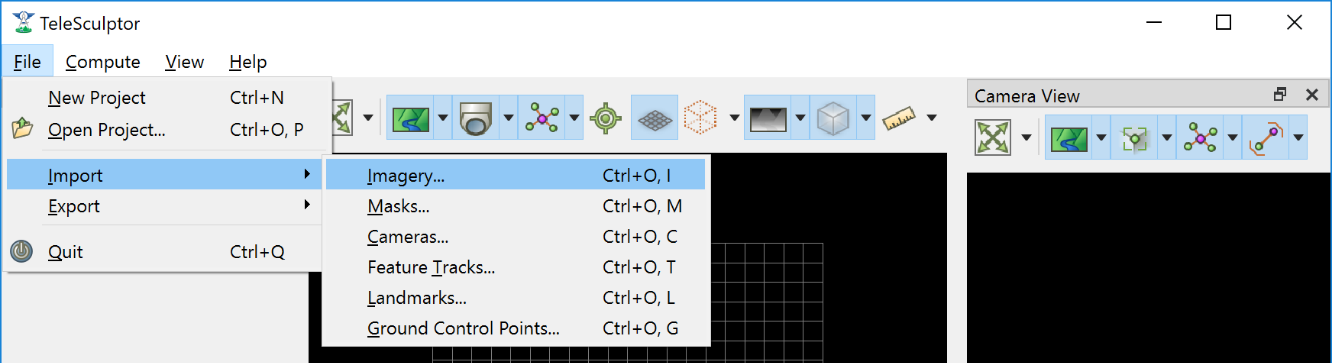
Import a video clip, image list, or other data.
Once a video is selected to open, the application will scan the entire video to find all metadata. This may take several seconds or even minutes for very large videos. If scanning the video takes too long or it is known that the video does not contain metadata it is okay to cancel the metadata scanning using the “Cancel” option in the Compute menu. If metadata scanning is canceled, then no metadata will be used in any subsequent processing steps.
The first video frame will appear in the Camera View in the upper right. The World View (left) will show a 3D representation of the camera path and camera viewing frustums if
relevant metadata is found. When images are shown in the 3D world view, they are always projected using the active camera model onto this ground plane (indicated by the grid). The
image button ( ) toggles visibility of images in each view with an opacity slider in the drop-down menu below the button. For images to appear in the world view an
active camera model is required. An active camera model is a camera model for the currently selected video frame.
) toggles visibility of images in each view with an opacity slider in the drop-down menu below the button. For images to appear in the world view an
active camera model is required. An active camera model is a camera model for the currently selected video frame.
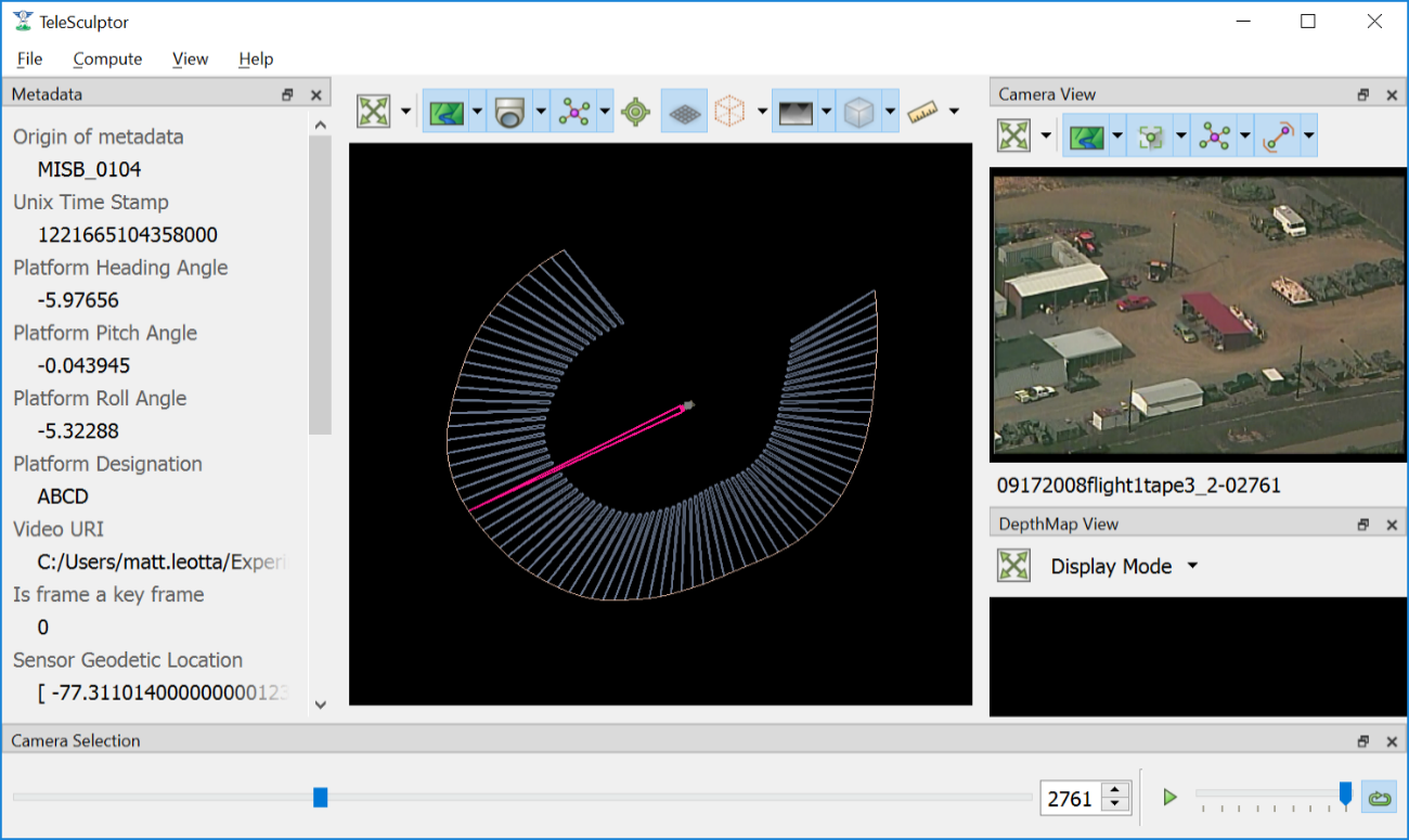
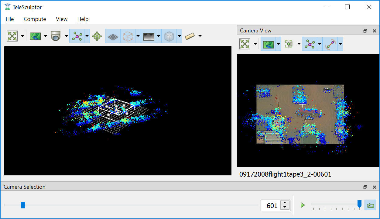
A video with KLV metadata opened in the application.
As can be seen in the image above. The aircraft flight path, as given in the metadata, is shown as a curved line in the 3D World View. A pyramid (frustum) is shown representing the orientation and position of the camera at each time step. The active camera, representing the current frame of video, is shown in a different color and is longer than the others. If the video is played with the play button in the lower right, the video frames will play in the Camera View and the active camera will updated in the World View.
The visibility of cameras is controlled by the cameras button ( ) above the world view. In the drop-down menu underneath the cameras button you can individually set
the visibility, size, and color of camera path, camera frustums, and active camera.
) above the world view. In the drop-down menu underneath the cameras button you can individually set
the visibility, size, and color of camera path, camera frustums, and active camera.
Run End-to-End
Run End-to-End is a new feature in TeleSculptor v1.2.0. Rather than waiting for user input to run each of the primary processing steps, Run End-to-End automatically runs Track Features, Estimate Cameras/Landmarks, Batch Compute Depth Maps, and Fuse Depth Maps. These steps are run sequentially in this order. See details of these steps in their respective sections below.

Run End-to-End Option in the Compute menu.
Track Features
The Track Features tool detects visually distinct points in the image called “features” and tracks the motion of those feature points through the video. This tool is run from the Compute menu and is enabled after creating a project and loading a video.
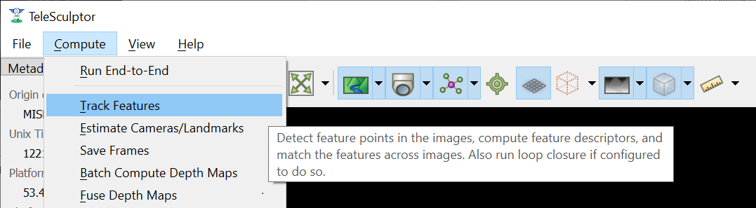
Run the Track Features algorithm from the Compute menu.
When the tool is running it will draw feature points on the current frame and slowly play through the video tracking the motion of those points as it goes. These tracks are
visualized as red trails in the image below. These colors are fully customizable. The feature tracks button (  ) above the Camera View enables toggling the
visibility of tracks. The drop-down menu under this button has settings for the display color and size of the feature track points and their motion trails.
) above the Camera View enables toggling the
visibility of tracks. The drop-down menu under this button has settings for the display color and size of the feature track points and their motion trails.
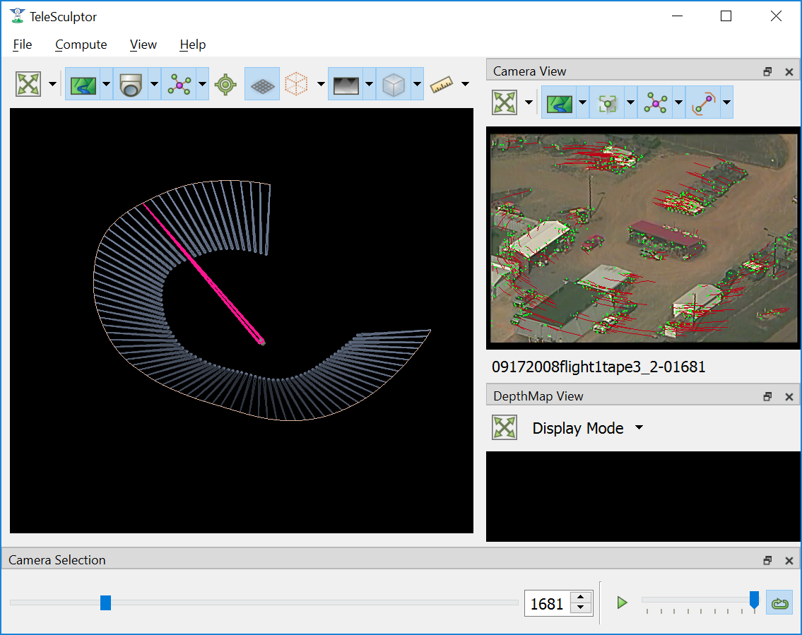
The Track Features algorithm producing tracks on a video.
The feature tracking tool will start processing on the active frame and will run until the video is complete or until the tool is canceled with the Cancel option in the Compute menu. We recommend starting with the video on frame 1 and letting the algorithm process until complete for a video clip containing approximately one orbit of the UAV above the scene. However, it is possible to process subsets of the video by scrubbing to a desired start frame before running the tool and then hitting the cancel button after reaching the desired end frame.
When this, or any other, tool is running all other tools will be disabled in the Compute menu until the tool completes. Most tools also support exiting early with the Cancel button to stop at a partial or suboptimal solution.
Note that to limit redundant computation this tool does not track features on every frame of video for long videos. Instead the algorithm sets a maximum of 500 frames (configurable in the configuration files) and if the video contains more than 500 frames it selects 500 frames evenly distributed throughout the video. Once feature tracking is done, tracks will flicker in and out when playing back the video due to frames with no tracking data. To prevent this flickering select Tracked Frames Only from the View menu. With this option enabled, playback is limited to frames which include tracking data.
More technical users who want to understand the quality of feature tracking results may wish to use the Match Matrix viewer under the View menu (keyboard shortcut M). The match matrix is a symmetric square matrix such that the value in the ith row and jth column is the number of features in correspondence between frames i and j. The magnitude of these value is colored with a color map and placing the mouse cursor over a pixel prints the actual number of matches in the status bar. Typically, a match matrix has strong response down the diagonal (nearby frames) that drops off as you move away from the diagonal. Flight paths that make a complete orbit should see a second weaker off-diagonal band where the camera returns to see the same view again.
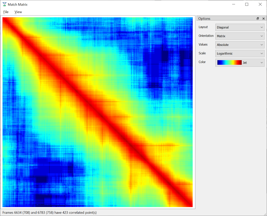
The Match Matrix view of feature tracking results.
Estimate Cameras/Landmarks
The Estimate Cameras/Landmarks tool in the Compute menu uses structure-from-motion algorithms to estimate the initial pose of cameras and the initial placement of 3D landmarks. It also uses bundle adjustment to jointly optimize both cameras and landmarks. These algorithms use the camera metadata as constraints and initial conditions when available. The algorithm will try to estimate a camera for every frame that was tracked and a landmark for every feature track.
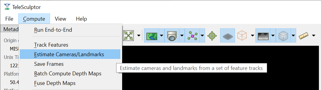
Run the Estimate Cameras/Landmarks algorithm from the Compute menu.
The solution will start with a sparse set of cameras and then incrementally add more. Live updates will show progress in the world view display. During optimization, the landmarks will appear to float above (or below) the ground plane grid because the true elevation is typically not near zero. Once the optimization is complete, a local ground height is estimated, and the ground plane grid is moved to meet the landmarks. This ground elevation offset is recorded as part of the geo-registration local coordinate system.
Once landmarks are computed their visibility can be toggled with the landmarks button (  ) in both the world and camera views. The drop-down menu under the
landmarks button allows changing the size and color of the landmarks including color by height or by number of observations.
) in both the world and camera views. The drop-down menu under the
landmarks button allows changing the size and color of the landmarks including color by height or by number of observations.
Save Frames
The Save Frames tool is quite simple. It simply steps through the video and writes each frame of video to disk as an image file. These image files are stored in a subdirectory of the project directory. Saving frames only requires an open video and an active project. It can be run at any time. Like the feature tracking tool, it plays through the video as it processes the data and can be cancelled to stop early. The primary purpose for saving frames is for using them in the TeleSculptor / SketchUp workflow. SketchUp can only load image images, not video. So, this step produces the image files that are needed when loading a project file into SketchUp.
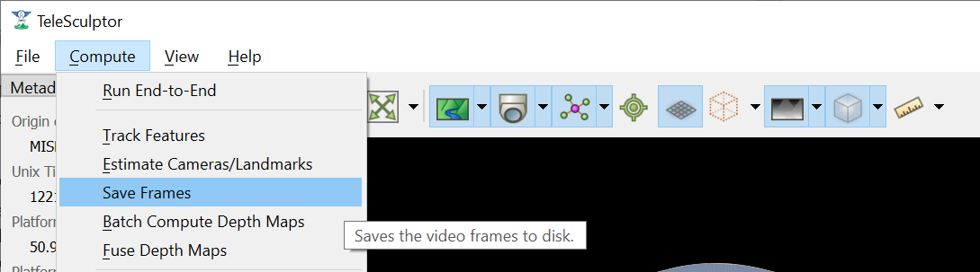
Save the loaded video frame as image files on disk.
Set Ground Control Points
Ground Control Points (GCPs) are user specified 3D markers that may be manually added to the scene for a variety of purposes. These markers are completely optional features that may be used to provide meaningful guide points for modeling when exporting to SketchUp. GCPs are also used to estimate geo-localization of videos with metadata or to improve geo-location for video with metadata.
To add GCPs press the GCP button (  ) above the 3D World View. To create a new GCP hold the Ctrl key on the keyboard and left click in either the 3D World View or the
2D Camera View. A new GCP will appear as a green cross in both views. Initial points are currently dropped into the scene along the view ray under the mouse cursor at the depth of
the closest scene structure. If the initial depth of a GCP is not accurate enough it can be moved. To move a point, left click on the point in either view and drag it. Points
will always move in a plane parallel to the image plane (or current view plane). It helps to rotate the 3D viewpoint or scrub the video to different camera viewpoints to correct the
position along different axes. Holding Shift while clicking and dragging limits motion to single coordinate axis. The axis of motion is the direction which has the most motion in
the initial mouse movement. Once additional points are added (with Ctrl + left clicks) the active point is always shown in green while the rest are shown in white. Left clicking
on any point makes it active. Hitting the Delete key will delete the current active GCP.
) above the 3D World View. To create a new GCP hold the Ctrl key on the keyboard and left click in either the 3D World View or the
2D Camera View. A new GCP will appear as a green cross in both views. Initial points are currently dropped into the scene along the view ray under the mouse cursor at the depth of
the closest scene structure. If the initial depth of a GCP is not accurate enough it can be moved. To move a point, left click on the point in either view and drag it. Points
will always move in a plane parallel to the image plane (or current view plane). It helps to rotate the 3D viewpoint or scrub the video to different camera viewpoints to correct the
position along different axes. Holding Shift while clicking and dragging limits motion to single coordinate axis. The axis of motion is the direction which has the most motion in
the initial mouse movement. Once additional points are added (with Ctrl + left clicks) the active point is always shown in green while the rest are shown in white. Left clicking
on any point makes it active. Hitting the Delete key will delete the current active GCP.
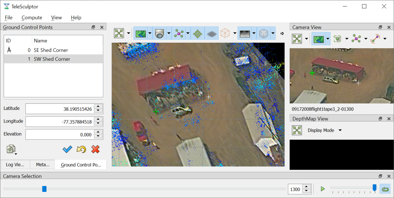
Setting ground control points. The active point is shown in green.
The Ground Control Points pane provides a way to select and manage the added GCPs. The pane lists all added points and allows the user to optionally assign a name to each. The GCP
pane also shows the geodetic coordinates of the active point, and these points can be copied to the clipboard in different formats using the copy location button
(  ). If the value of the geodetic coordinates is changed that GCP becomes a constraint and is marked with an icon (
 ![]() ) in the GCP list. Constrained
points will keep fixed geodetic coordinates when the GCP is moved in the world space. A constraint can be removed by pressing the reset button (
) in the GCP list. Constrained
points will keep fixed geodetic coordinates when the GCP is moved in the world space. A constraint can be removed by pressing the reset button (  ). Once at least
three GCP constraints are added with geodetic coordinates, the apply button (
). Once at least
three GCP constraints are added with geodetic coordinates, the apply button (  ) can be used to estimate and apply a transformation to geolocalize the data. While
three GCPs are the minimum, five or more are recommended. The transformation will be fit to all GCP constraints. After applying the GCPs, all cameras, landmarks, depth maps, and
GCPs are transformed to the new geographic coordinates. Currently the mesh fusion is not transformed because the integration volume is axis-aligned. Instead the fusion results are
cleared and need to be recomputed.
) can be used to estimate and apply a transformation to geolocalize the data. While
three GCPs are the minimum, five or more are recommended. The transformation will be fit to all GCP constraints. After applying the GCPs, all cameras, landmarks, depth maps, and
GCPs are transformed to the new geographic coordinates. Currently the mesh fusion is not transformed because the integration volume is axis-aligned. Instead the fusion results are
cleared and need to be recomputed.
It is often helpful to compute a depth map (or even fused 3D model) before setting GCPs to provide additional spatial reference in the 3D view. It is possible set GCPs entirely from the 2D camera views by switching between video frames and correcting the position in each. However, this is more tedious. When the 3D position is correct the GCP should stick to the same object location as the video is played back.
GCPs are currently not saved automatically. To save the GCP state use the File->Export->Ground Control Points menu option and create a PLY file to write. This file path is cached in the project configuration, so GCPs are automatically loaded when the project is opened again. They are also automatically loaded when importing the project configuration into SketchUp.
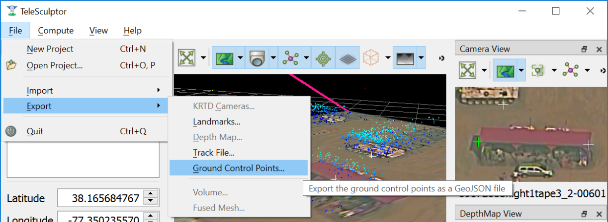
Export the ground control points.
Set 3D Region of Interest
Before running dense 3D modeling operations, it is beneficial to set a 3D region of interest (ROI) around the portion of the scene that is of interest. This step is optional. By default, a ROI is chosen to enclose most of the 3D landmark point that were computed in the triangulate landmarks step. Some outlier points are rejected when fitting the ROI and the estimated ROI is padded to account for missing data. The default ROI is generally sufficient for further processing, but may be larger than necessary. The advantage of picking a smaller ROI is a significant reduction in compute time and resources. Furthermore, the quality and resolution of the result often improves when focusing on smaller subset of a large scene because we can focus more compute resources on that location.
To see and manipulate the 3D ROI click the 3D ROI button (  ) above the 3D World View. A 3D axis-aligned box is shown which contains the set of 3D landmarks. Inside
the box are axis lines along the center of the box in each of the three coordinate directions. At the ends of these lines are spheres which act as manipulation handles. Left click
on any of these handles and drag to reposition the corresponding face of the box in 3D. Left click the sphere at the center of the box and drag to translate the entire box. A
middle click (or Ctrl + left click or Shift + left click) and drag anywhere in the box has the same translation effect as using the center handle. A right click and drag will
scale the box uniformily about its origin. Note that the ground plane grid will adjust size relative to the ROI size.
) above the 3D World View. A 3D axis-aligned box is shown which contains the set of 3D landmarks. Inside
the box are axis lines along the center of the box in each of the three coordinate directions. At the ends of these lines are spheres which act as manipulation handles. Left click
on any of these handles and drag to reposition the corresponding face of the box in 3D. Left click the sphere at the center of the box and drag to translate the entire box. A
middle click (or Ctrl + left click or Shift + left click) and drag anywhere in the box has the same translation effect as using the center handle. A right click and drag will
scale the box uniformily about its origin. Note that the ground plane grid will adjust size relative to the ROI size.
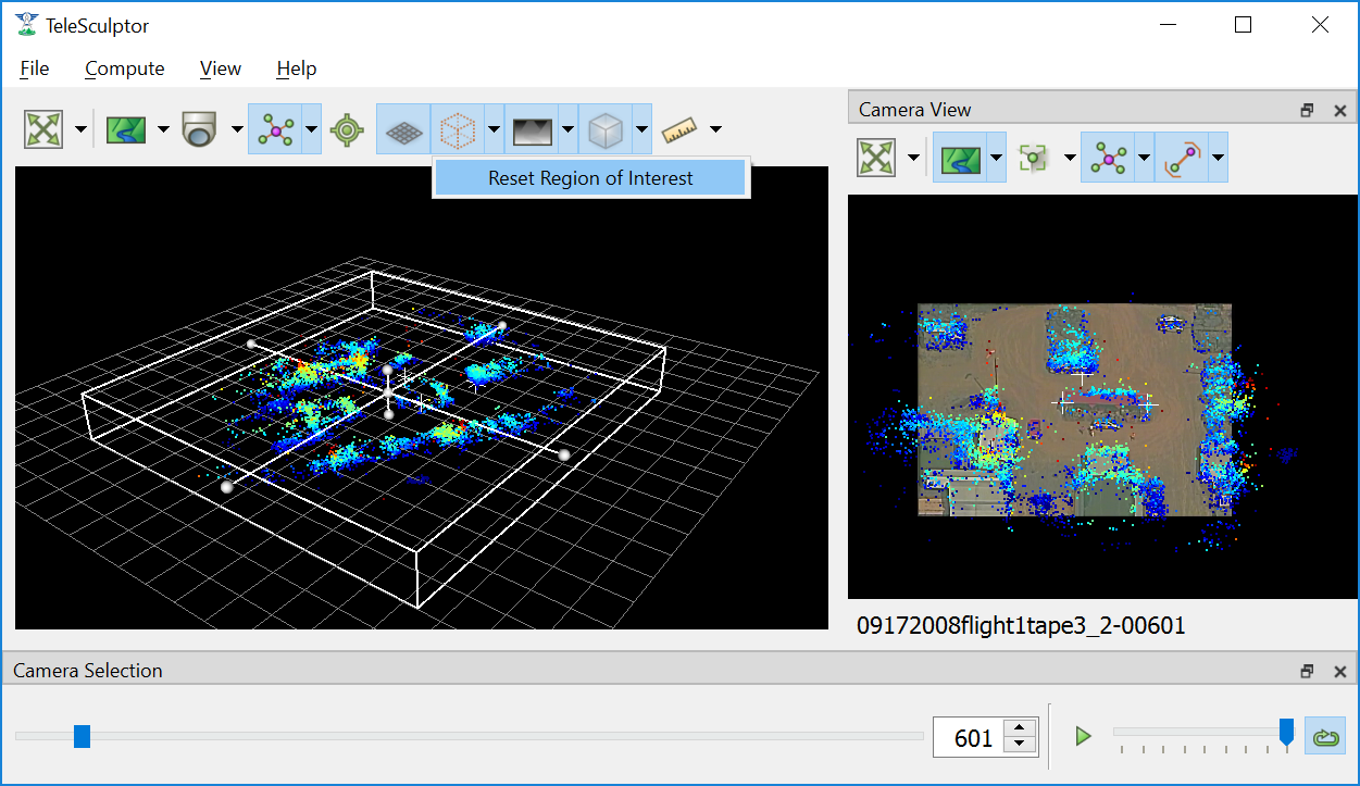
The default 3D bounding box is fit to the sparse landmarks and is often bigger than needed.
A good practice is to set the bottom of the ROI box just below the ground and the top just above the tallest part of the structure. Likewise, set the sides to be just a bit outside the object of interest. It may be difficult to determine the bounds accurately from the sparse landmarks. A good strategy is to start with a slightly larger guess, then use the Compute Single Depth Map advanced tool to compute a single depth map. The depth map gives more detail which helps pick a tighter box. Then use Batch Compute Depth Maps to compute the additional depth maps with the revised box.
To reset the ROI to the initial estimated bounding box, use the Reset Region of Interest option in the drop-down menu under the ROI button.
Setting a tighter bounding box around one structure of interest.
Batch Compute Depth Maps
Computation of dense depth maps is part of the fully automated 3D reconstruction pipeline. Several depth maps are needed to compute a final 3D result. Running the Batch Compute Depth Map tool from the Compute menu will estimate depth maps (2.5D models) for twenty different frames sampled evenly through the video. To compute a depth map only on the current frame, see the Compute Single Depth Map option in the advanced menu.
This algorithm requires very accurate camera and landmark data resulting from the previous Estimate Cameras/Landmarks step above. Furthermore, cameras models on multiple frames in nearby positions are required. By default, the algorithm uses the ten frames before and ten frames after each selected depth frame for reference.
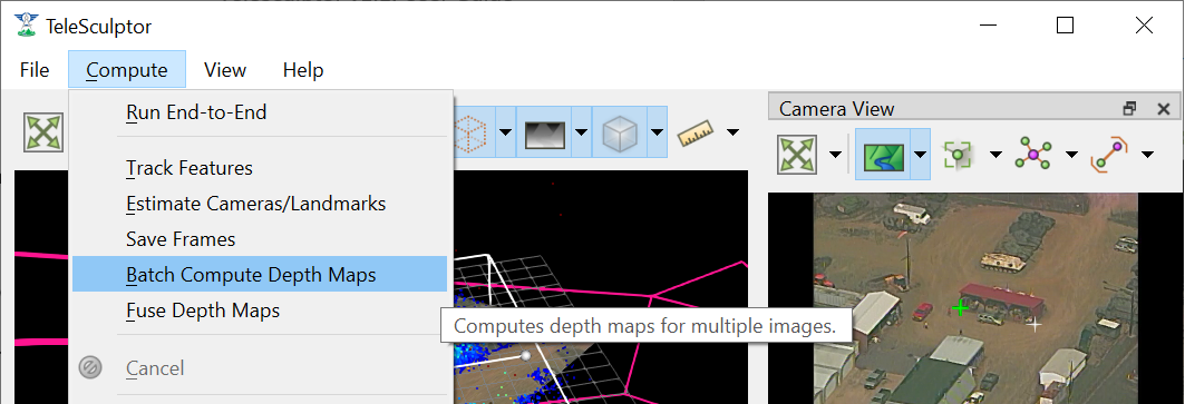
Compute dense depth maps on key frames.
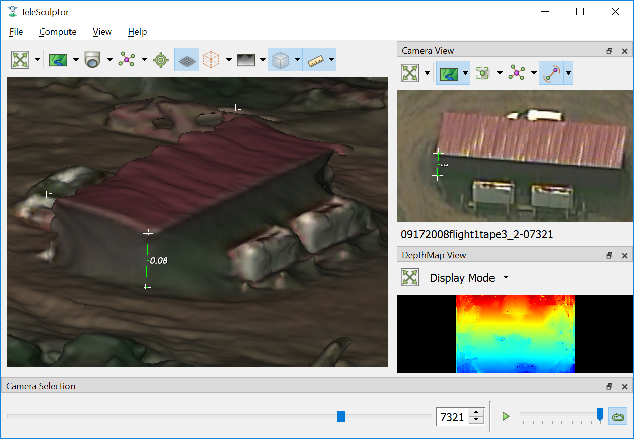
The results of depth map estimation are shown in two ways. In the world view the depth maps are shown as a dense colored point cloud in which every image pixel is back projected
into 3D at the estimated depth. Use the Depth Map button (  ) to toggle depth point cloud visibility. The second way depth maps are visualized is as a depth image
in the Depth Map View. Here each pixel is color coded by depth and the color mapping is configurable.
) to toggle depth point cloud visibility. The second way depth maps are visualized is as a depth image
in the Depth Map View. Here each pixel is color coded by depth and the color mapping is configurable.
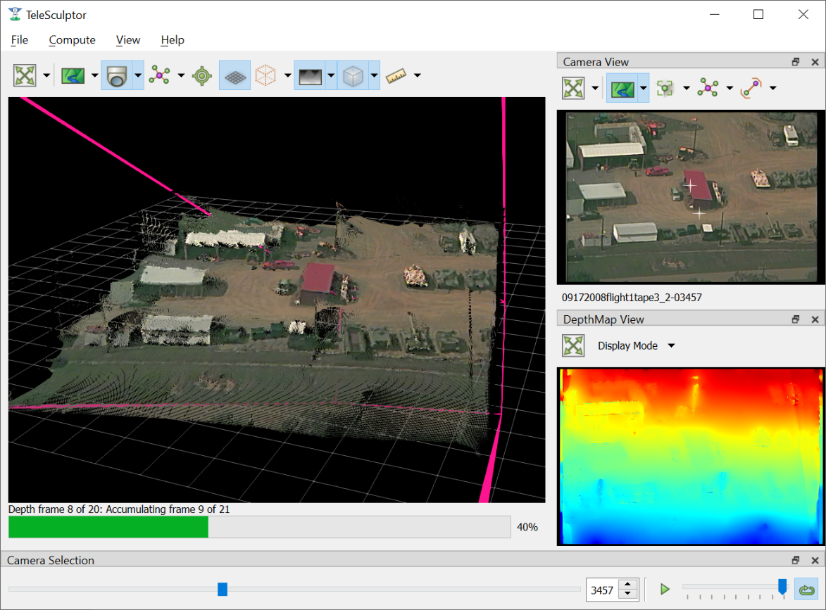
Results of depth map computation.
Fuse Depth Maps
After computing depth maps in batch, or manually computing multiple depth maps, the next step is to fuse them into a consistent 3D surface. Running Fuse Depth Maps from the Compute menu will build an integration volume and project all depth maps into it for fusion. This integration step requires a modern CUDA capable Nvidia GPU (Requires at least Nvidia driver version 396.26). The size of the integration volume and the ROI covered is determined by the same ROI box used in the depth map computation. This processing step runs in only a few seconds and may cause lag in the display during this time due to consumption of GPU resources. Once the data is fused into a volume, a mesh surface is extracted from the volume.
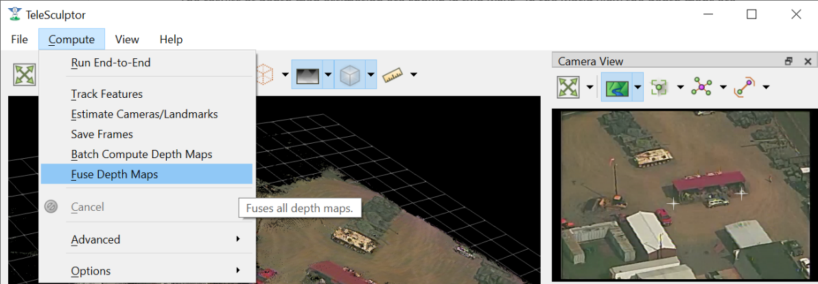
Fuse the depth maps into a consistent mesh.
To toggle the view of the fused mesh, press the Volume Display button (  ) above the 3D World View. The surface mesh can be fine-tuned if desired by adjusting
the surface threshold in the drop-down menu under the Volume Display button. Setting the threshold slightly positive (e.g. 0.5) often helps to remove unwanted outlier surfaces that
tend to appear in areas with only a few views.
) above the 3D World View. The surface mesh can be fine-tuned if desired by adjusting
the surface threshold in the drop-down menu under the Volume Display button. Setting the threshold slightly positive (e.g. 0.5) often helps to remove unwanted outlier surfaces that
tend to appear in areas with only a few views.
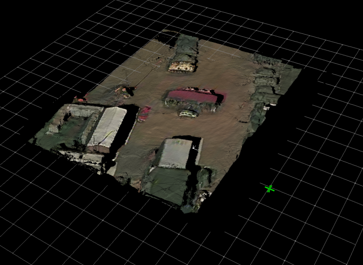
View the fused mesh, adjust surface threshold if desired.
Colorize Mesh
The fused mesh is provided initially in a solid grey color.
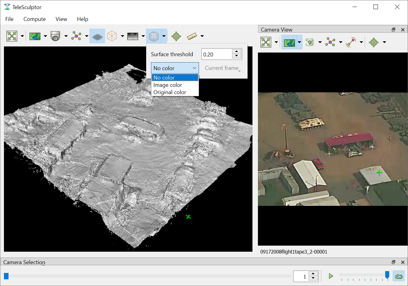
To add color, use the drop down menu under the
Volume Display button ( ).
Use the left drop down menu to select between No Color and Image Color.
If, and only if, a mesh was loaded from a file,
a third option for Original Color is available.
Original Color displays the color loaded from the mesh file.
The mesh colorization menu options.
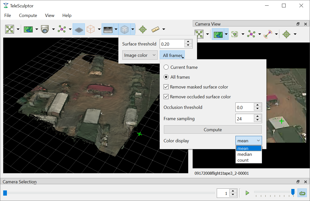
If Image Color is selected then the mesh vertices are colored by projecting color from one or more images onto the mesh. Additional settings on how the mesh is colored are in the right drop down menu. The Current frame option always projects the current frame onto the mesh and the color updates when you play back the video. The All frames option estimates a static mesh coloring by projecting multiple images onto the surface and combining them. The Frame sampling combo box allows configuration of how frequently to sample frames for coloring. Smaller sampling uses more frames for better color but more computation time. Press the Compute button to compute mesh color. When complete, the Color display option can be changed without needing to recompute color. The recommended color display option is median, however, mean is often quite similar. The count option colors by the number of depth map views that observed each part of the surface.
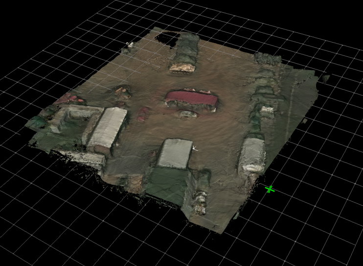
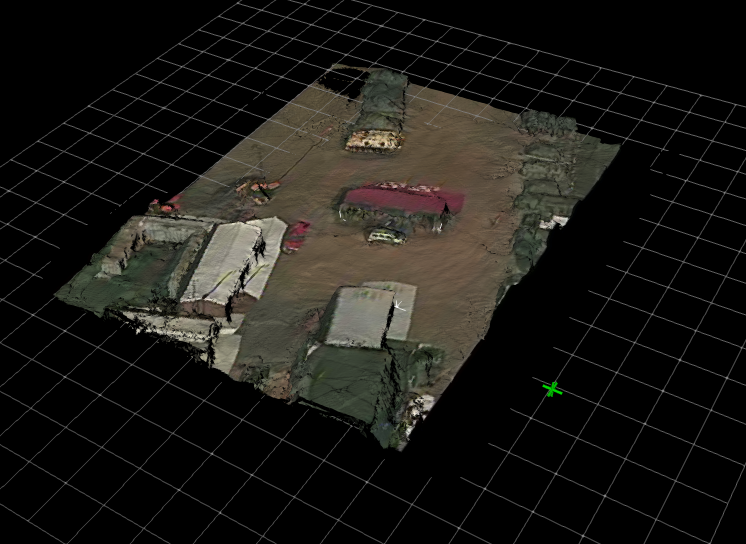
A fused mesh colored by the mean of multiple frames.
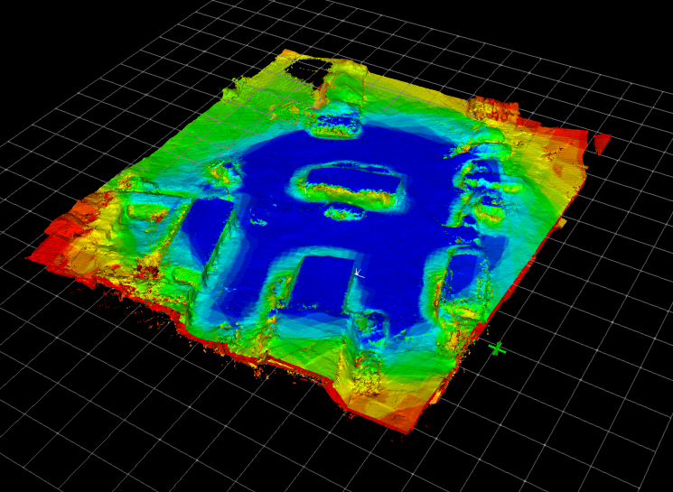
A fused mesh colored by the number of views that see each part of the surface.
Additional check boxes are available to enable removal of color on some surfaces that should not be colored. The Remove masked surface color option uses a mask video loaded into TeleSculptor and does not apply color at points under this mask. The Remove occluded surface color option enables visibility checking such that occluded surfaces will not receive color. The Occlusion threshold varies the sensitivity of the occlusion depth test. Negative values cause larger occluded regions while positive values cause smaller occluded regions.
A fused mesh colored by a single frame using occlusion detection.
A fused mesh colored by a single frame without occlusion detection.
Export Data
To export the finale colorized mesh for use in other software, use the File->Export->Fused Mesh menu item. This will provide a file dialog to save the model as a mesh in standard PLY, OBJ, LAS, or VTP file formats. The LAS file format will only save the dense mesh vertices as a point cloud and does include geo-graphic coordinates. The other formats save the surface mesh but only in local coordinates. Note that all formats (except OBJ) will also save RGB color on the mesh vertices. This color matches whatever display options are currently set.
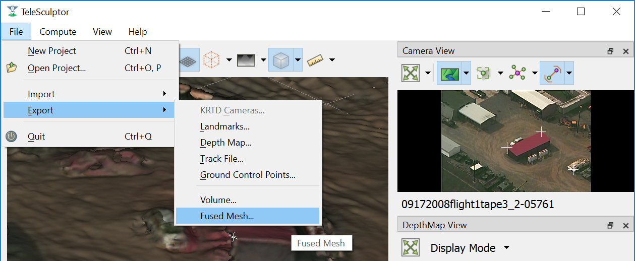
Save a colorized mesh as a PLY, LAS, or VTP file.
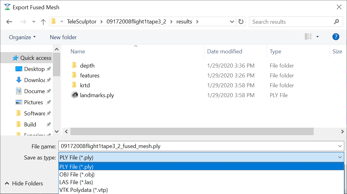
Change the Save as type to export as LAS.
To export the active 2.5D depth map for use in other software, use the File->Export->Depth Map menu item. This will provide a file dialog to save the model as an RGB colored point cloud in the standard PLY or LAS file formats.
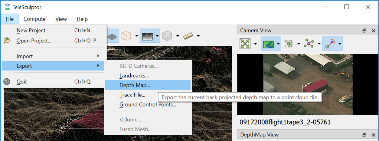
Save a computed depth map as a point cloud in PLY or LAS formats.
Measurement Tool
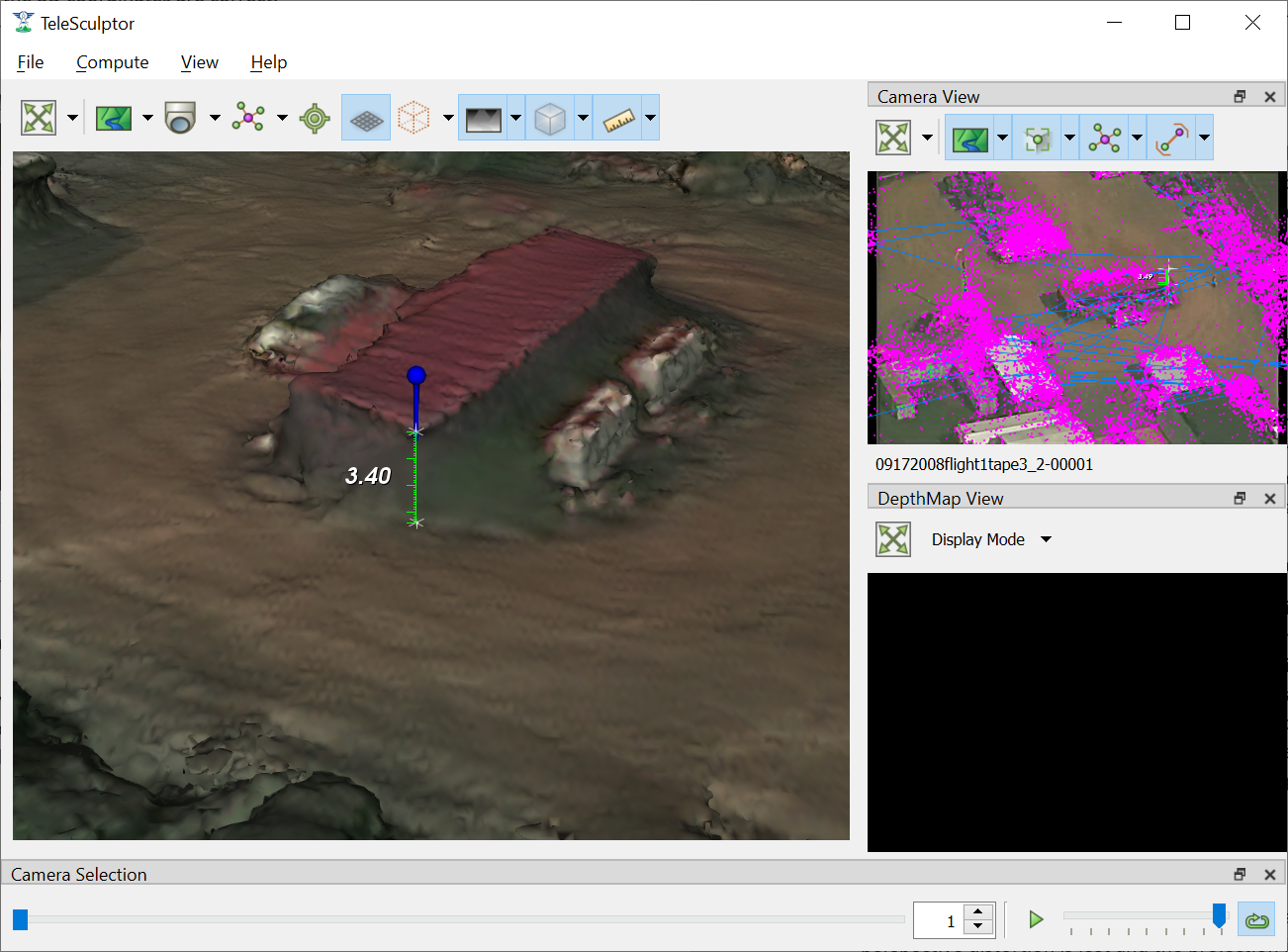
The measurement tool (  ) allows the user to measure straight line distance in world coordinates. Placing the end points of the ruler uses a similar interface to
placing GCPs, and each end point can be adjusted independently just like GCPs. The number displayed next to the green line in both world and camera views represents the distance in
world space. If geo-spatial metadata is provided the measurements are in units of meters. Without metadata (as in the example below) the measurements are unitless. The ruler can
be drawn and adjusted in either the world or camera views. Often it is easier to get more accurate alignment in the image space. As with GCPs, if the ruler sticks to the correct
location when playing back the video then the 3D coordinates are correct.
) allows the user to measure straight line distance in world coordinates. Placing the end points of the ruler uses a similar interface to
placing GCPs, and each end point can be adjusted independently just like GCPs. The number displayed next to the green line in both world and camera views represents the distance in
world space. If geo-spatial metadata is provided the measurements are in units of meters. Without metadata (as in the example below) the measurements are unitless. The ruler can
be drawn and adjusted in either the world or camera views. Often it is easier to get more accurate alignment in the image space. As with GCPs, if the ruler sticks to the correct
location when playing back the video then the 3D coordinates are correct.
Measuring a building height with the measurement tool.
When measuring it is sometimes convenient to constraint the measurements to the horizontal or vertical directions. After the initial ruler is placed in the scene, click and drag one end point. If the Z key is held on the keyboard the moving point will be constrained to lie on a vertical axis through the point at the other end of the ruler. If either the X or Y keys is held, the moving point will be constrained to lie in a horizontal (X-Y) plane that passes through the other ruler point. Each of these constraints is indicated by an indicator as shown below.
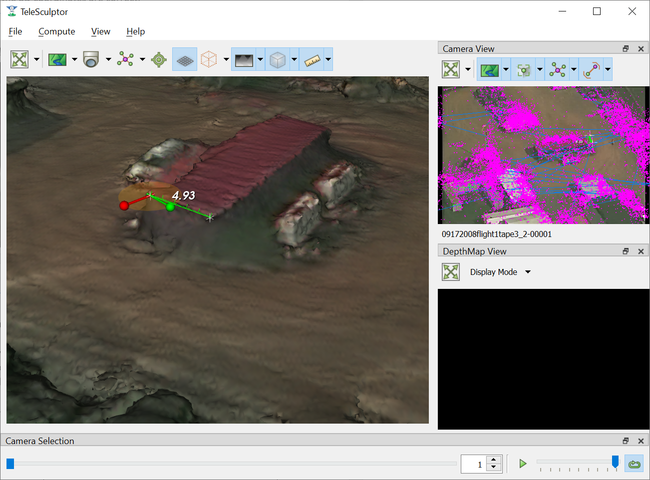
Vertical Constraint (hold Z) Horizontal Constraint (hold X or Y)